


Sophisticated adversaries are moving their botnet command and control infrastructure to social media microblogging sites such as Twitter. As security practitioners work to identify new methods for detecting and disrupting such botnets, including machine-learning approaches, we must better understand what effect training data recency has on classifier performance.
This research investigates the performance of several binary classifiers and their ability to distinguish between non-verified and verified tweets as the offset between the age of the training data and test data changed. Classifiers were trained on three feature sets: tweet-only features, user-only features, and all features. Key findings show that classifiers perform best at +0 offset, feature importance changes over time, and more features are not necessarily better. Classifiers using user-only features performed best, with a mean Matthews correlation coefficient of 0.95 ± 0.04 at +0 offset, 0.58 ± 0.43 at -8 offset, and 0.51 ± 0.21 at +8 offset. The R2 values are 0.90, 0.34, and 0.26, respectively. Thus, the classifiers tested with +0 offset accounted for 56% to 64% more variance than those tested with -8 and +8 offset. These results suggest that classifier performance is sensitive to the recency of the training data relative to the test data. Further research is needed to replicate this experiment with botnet vs. non-botnet tweets to determine if similar classifier performance is possible and the degree to which performance is sensitive to training data recency.
Introduction
Botnets are using increasingly sophisticated methods not only to communicate but to conceal the presence of the botnet communication. Covert command and control channels make it more difficult to detect and disrupt botnet communication, one of the most common methods for disabling a botnet. Can modern machine learning techniques identify social media messages (tweets) associated with covert botnet command and control traffic? And if so, to what extent is the performance of such classifiers dependent on having recent training data? I selected tweet- and user-specific features of tweets and trained a variety of binary classifiers to distinguish between non-verified and verified tweets, then measured their performance when predicting the non-verified vs. verified status of tweets from a range of years. Developing a better understanding of how classifiers can distinguish between “trusted” and “untrusted” classes of tweets will lead to better techniques for detecting and disrupting covert botnet command and control channels. Understanding the impact of training data recency will lead to the creation of more effective classifiers.
Literature Review
Botnets are massive, distributed networks of bots or zombies, typically seen in the form of malware-infected hosts – that is, unwitting participants (Bailey, Cooke, Jahanian, Xu, & Karir, 2009; Vania, Meniya, & Jethva, 2013). Botnets rely on a command and control (C&C) channel to receive, execute, and respond to commands from the botmaster (Bailey et al., 2009; Vania et al., 2013). Over time, botnets have become more sophisticated, employing cutting-edge techniques to maintain availability and evade detection. In the early days of botnets, circa 2000, botnets relied on Internet Relay Chat (IRC) for C&C. IRC afforded a centralized command structure, anonymity, one-to-one (private) communication, and one-to-many communication (Vania et al., 2013). System administrators responded by restricting and monitoring access to IRC. Botnets, in turn, moved to a peer-to-peer (P2P) C&C structure, in which there is no central server; bots instead received commands from trusted locations or peers (other bots) (Bailey et al., 2009; Vania et al., 2013). Detecting such P2P botnets is difficult, and became more so with the advent of fast-flux botnets. Traditional approaches to detecting P2P botnets focus on network analysis – classifying traffic based on endpoints, latency, frequency, synchronicity, packet size, and similar (Bailey et al., 2009). The next evolution in botnet C&C was to move to social media and microblogging platforms, such as Facebook and Twitter (Kartaltepe, Morales, Xu, & Sandhu, 2010; Rodríguez-Gómez, Maciá-Fernández, & García-Teodoro, 2013; Stamp, Singh, H. Toderici, & Ross, 2013). The advantages of this move are that such platforms are resilient (their business depends on it), high-volume, and accessed over HTTP/HTTPS.
Moving to social media effectively hides C&C traffic amongst the noise of legitimate traffic, making it impossible to block outright (Kartaltepe et al., 2010; Stamp et al., 2013). Instead, defenders are forced to distinguish the C&C traffic from the legitimate traffic. Jose Nozario, a research scientist with Arbor Networks, documented a naïve approach to C&C over Twitter (2009) in which the botmaster issued commands via tweet, with each tweet containing a base64 encoded bit.ly link. The links, in turn, contained base64 encoded executables. Such a C&C approach is obvious to anyone that is watching, as base64 encoded messages stand out from typical Twitter traffic. Stegobot uses image steganography to hide the commands in images, which it then posts to social media – Facebook in this case – to conceal the presence of the command (Nagaraja et al., 2011). In Covert Botnet Command and Control Using Twitter, Pantic and Husain proposed an approach to concealing the presence of command and control traffic by using noiseless steganography and encoding the commands in the metadata – message length in this case (Pantic & Husain, 2015).
Disrupting a botnet requires either disabling the botmaster, disabling the zombies, cleaning the botnet malware from the zombies, or interfering with the ability of the botmaster to communicate with the zombies (Gu, Zhang, & Lee, 2008). Ten years ago, interfering with the C&C channel could be as simple as blocking all outbound IRC traffic from a network. Botnet detection focused on host-based or network-based analysis techniques (Cooke, Jahanian, & McPherson, 2005). The use of a legitimate social media platform as a covert C&C channel has complicated this. Research has been conducted on detecting Twitter spam accounts (Hua & Zhang, 2013) and classifying accounts as either human, bot, or cyborg (human-assisted bots or bot-assisted humans) (Chu, Gianvecchio, Wang, & Jajodia, 2010) using machine learning. In Detection of Stegobot: a covert social network botnet, Natarajan, Sheen, and Anitha (2012) presented a method for detecting Stegobot activity by analyzing the entropy of cover images, but there is still a research gap in the detection of botnet C&C behavior in Twitter. This gap is due at least in part to an acute lack of high-quality labeled training data, but this will hopefully change as researchers continue to identify large botnets in the wild, such as the 350,000 node botnet discovered by researchers at University College in London (Echeverría & Zhou, 2017). But the eventual availability of more and higher quality data leads to another research question: how important is the recency of the training data relative to the behaviors of interest? In other words, is there an expiration date on training data?
Research Method
The experiment required collecting and processing approximately 3.9 million tweets. From those, 1,500 tweets (1,000 non-verified and 500 verified) were randomly sampled from each year, 2010 – 2018, to generate nine datasets. For each year, several classifiers were trained with 1,000 tweets randomly sampled from that year’s dataset. Based on the analysis conducted, there was no measurable increase in performance when training with more than 1,000 tweets per year. Classifiers were then evaluated against each year individually. Test sets were generated by randomly sampling 300 tweets (200 non-verified and 100 verified). The same training and test datasets were used for each classifier. To evaluate classifiers against their own year, tweets were drawn from the 500 tweets not used to train the classifier. To evaluate classifiers against other year data, the tweets were drawn from the entire dataset. This approach guaranteed that classifiers were not trained and evaluated using the same tweets.
Data Collection
Twitter introduced the Verified designation in June 2009. The initial analysis determined that the percentage of non-verified vs. verified tweets is highly imbalanced. As of March 2018, the data collected for this experiment shows that only 0.08% of Twitter users are verified, and 5% of tweets are from verified users. To address this, the data were oversampled without replacement, with a final distribution of 67% non-verified tweets and 33% verified tweets. However, the Twitter API limits access to only the 3,200 most recent tweets for each user. This makes it challenging to collect sufficient data for prior years. For example, of the 1,633 users in the final dataset, only 37 had one or more tweets in 2010. Of the 3.9 million tweets collected, 2,456 are from 2010. This is why it was necessary to collect such a large number of tweets to end up with a comparatively small dataset.
Data Processing
The Twitter API returns statuses as JSON objects. These JSON objects were then converted to comma-separated value (CSV) files. Some fields, such as retweeted_status, were converted to a boolean representation based on whether the field was present in the JSON object. Boolean values were converted to an integer value 0 (false) or 1 (true). Table 1 summarizes the JSON fields, corresponding CSV fields, Python data type, and default value used (if any). Table 2 summarizes the additional fields that were derived from the fields in Table 1.
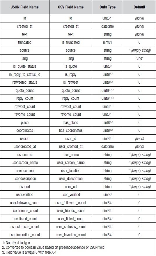
Table 1: JSON and CSV Data Fields
Classifier Training
After data processing, the entire set of 3.9 million tweets was split into nine disjoint sets based on the created_at field year: 2010, 2011, 2012, 2013, 2014, 2015, 2016, 2017, and 2018. For each year, a subset was created by randomly sampling 1,000 non-verified tweets and 500 verified tweets. This subset was then randomly split into a training set and a validation set, comprising 67% and 33% of the subset respectively. For each training set, the scikit-learn Imputer preprocessor was fitted to NaN values using the mean strategy and the RobustScaler preprocessor was fitted with default parameters. Finally, each classifier was fitted to the training data using default parameters.
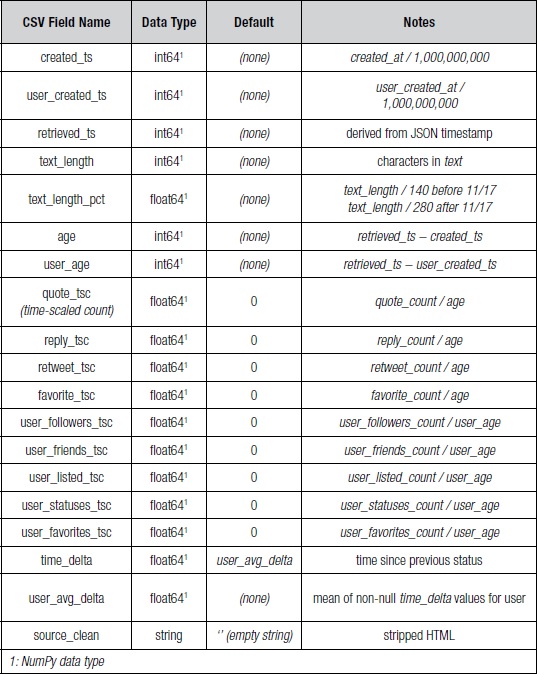
Table 2: Derived Fields
Classifier Evaluation
Initial experimentation showed that classifiers performed extremely well by predicting that all tweets are non-verified. While accurate, this finding was of limited value. If 95% of tweets are from non-verified users and 5% are from verified users, a classifier would achieve 95% accuracy by predicting that all tweets are non-verified. This necessitated changing the performance metric from accuracy to Matthews correlation coefficient (MCC). MCC was chosen as it incorporates true positives (TP), true negatives (TN), false positives (FP), and false negatives (FN). The formula is as follows:


MCC is considered a balanced measure that performs well with imbalanced data classes (Boughorbel, Jarray, & El-Anbari, 2017). In the scenario where 95% of tweets are from non-verified users and 5% are from verified users, predicting that all tweets are non-verified would result in an MCC value of 0 (no correlation).
Each trained classifier was evaluated against each year from 2010 to 2018. For each year, a test set was created by randomly sampling 200 non-verified tweets and 100 verified tweets from the full dataset for the year. The exception to this was when the training year and test year were equal, in which case the validation set was used as the test set. Each test set was transformed using the previously fitted Imputer and RobustScaler preprocessors. Finally, the test class (non-verified vs. verified) was predicted using the previously fitted classifier and the MCC was calculated.
Potential Shortcomings
While care was taken to avoid common mistakes such as training and testing using the same data, the nature of the Twitter API does present some challenges. Chief among these is a potential selection bias. Twitter does not provide a method to choose a random user ID, so random user IDs were selected from a sample of the live stream, which means that all tweets used in this experiment are from users that were active as of March 2018.
Second, the Twitter API only provides the 3,200 most recent Tweets for each user. This means that the more active a user is, the more recent the cutoff. Consequently, data from more distant years are more likely to be from less active users.
Findings and Discussion
Feature Importance
Each classifier was trained and evaluated with three features sets: tweet-only features, user-only features, and all features.
Tweet-only features are specific to an individual tweet and do not include user information. The following features were included: created_ts, age, time_delta, is_truncated, is_quote, is_reply, is_retweet, has_place, has_coordinates, text_length, text_length_pct, quote_tsc, reply_tsc, retweet_tsc, and favorite_tsc.
User-only features are independent of individual tweets and represent a user at the time the tweet is retrieved, not at the time the tweet is originally posted. The following features were included: user_created_ts, user_age, user_followers_tsc, user_friends_tsc, user_listed_tsc, user_statuses_tsc, user_favorites_tsc, user_avg_delta.
All features combines the features from the tweet-only and user-only feature sets.
The mutual information (MI) score for each feature was calculated to determine how strongly the feature contributed to the correct classification. This information was not used for feature selection, but rather to measure the relative importance of features. Figure 1 is a plot of the mean and standard deviation per year of the tweet-only vs. user-only feature sets.
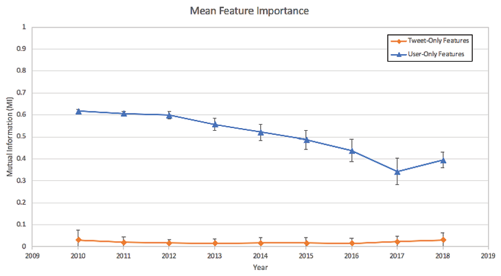
Figure 1: Feature importance for tweet-only vs. user-only feature sets
The mean mutual information scores for the user-only features are 14 to 20 times higher than those for tweet-only features. This means that user-only features are stronger indicators of whether a tweet is non-verified vs. verified, a conclusion that will be confirmed when classifier performances are examined.
The mean mutual information scores for user-only features drop steadily over time. One possible explanation for this observation is that user characteristics and behaviors have become less able to predict if a tweet is from a verified user as the Twitter user base has grown in size and diversity.
Classifier Performance
The experiment compares the performance of seven classifiers: k-nearest neighbors, logistic regression, SVC, multi-layer perceptron, decision trees, random forest, and gradient boosting. In each instance, the scikit-learn implementation with default parameters was used. No optimization was performed.
For the purposes of evaluating classifier performance, the data has been offset such that the difference between training year and test year are the same at a given point on the x-axis. For example, Figure 2 shows MCC values for the SVC classifier with user-only features. In the top table, the y-axis represents the training data year and the x-axis represents the test data year. However, this research is primarily focused on determining how well classifiers can predict the class of data that is older or newer than the training data. In the bottom table, the data has been shifted to reflect the offset between the test year and the training year. In the first row, which corresponds to training data from 2010, the test data from 2010 has an offset of +0 (2010 – 2010), the test data from 2011 has an offset of +1 (2011 – 2010), and so on. As a result, we can quickly see that for an offset of +0 (that is, for all instances in which the training data year and test data year were the same), the performance was quite good, but declines as the offset grows. This approach to offsetting the data is used throughout this paper.

Figure 2: Example of performance data before and after being offset
Tweet-Only Features
Figure 3 compares the individual mean Matthews correlation coefficient of seven different classifiers.
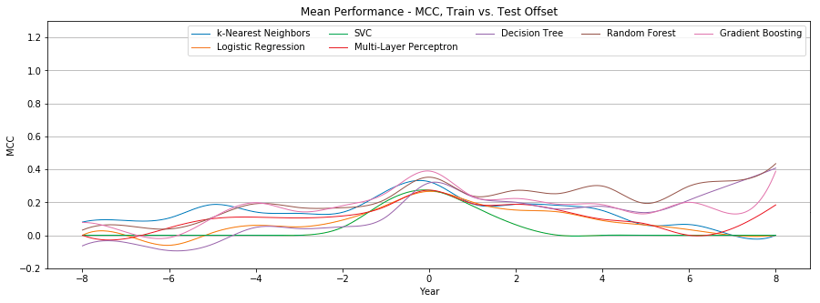
Figure 3: Mean performance of each classifier with tweet-only features
Figure 4 shows the mean Matthews correlation coefficient and standard deviation of all seven classifiers. Performance is optimal at +0 offset, with a mean MCC of 0.31 ± 0.04 (weak positive relationship), and quickly drops as the offset changes. After reaching a low of 0.09 ± 0.06 at +5 offset, the MCC begins to rise, but so does the standard deviation, until reaching an MCC of 0.2 ± 0.19.
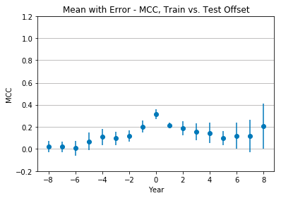
Figure 4: Mean classification performance across all classifiers with tweet-only features
User-Only Features
Figure 5 compares the individual mean Matthews correlation coefficient of seven different classifiers.
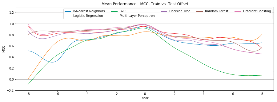
Figure 5: Mean performance of each classifier with user-only features
Figure 6 shows the mean Matthews correlation coefficient and standard deviation of all seven classifiers. Again, performance is optimal at +0 offset, with a mean MCC of 0.95 ± 0.04 (very strong positive relationship), and drops as the offset changes. Unlike the tweet-only features, however, performance at the extreme offsets still shows a moderate positive relationship. At -8 offset the mean MCC is 0.58 ± 0.43, while at +8 offset the mean MCC is 0.51 ± 0.21. In both instances, the standard deviation grows as we move from an offset of +0.
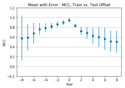
Figure 6: Mean classification performance across all classifiers with user-only features
All Features
Figure 7 compares the individual mean Matthews correlation coefficient of seven different classifiers.
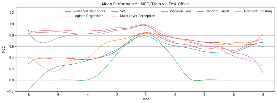
Figure 7: Mean performance of each classifier with user-only features
Figure 8 shows the mean Matthews correlation coefficient and standard deviation of all seven classifiers. Again, performance is optimal at +0 offset, with a mean MCC of 0.89 ± 0.08 (very strong positive relationship) and drops as the offset changes. Performance at the extreme offsets still shows a moderate positive relationship, though not to the same extent as with the user-only features. At -8 offset the mean MCC is 0.4 ± 0.41, while at +8 offset the mean MCC is 0.45 ± 0.3. In both instances, the standard deviation grows as we move from an offset of +0.
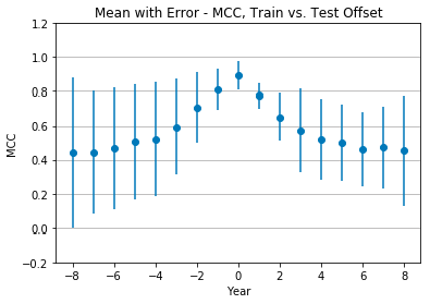
Figure 8: Mean classification performance across all classifiers with all features
Summary of Findings
The experiment resulted in three key findings:
- Classifiers perform best at +0 year offset and generally perform worse as the offset increases or decreases. Ensemble classifiers (random forest, gradient boosting), decision trees, and multi-layer perceptron were most resilient to this performance loss. For these four classifiers, the mean MCC at +0, -8, and +8 offset was 0.98 ± 0.01, 0.91 ± 0.08, and 0.51 ± 0.06 respectively. SVC was the most susceptible to performance loss, with mean MCC at +0, -8, and +8 offset of 0.92, -0.097, and 0.07 respectively. This finding suggests that it is important to use recent training data and that different classifiers are more or less sensitive to this recency requirement.
- Feature importance changes over time. The tweet-only features were uniformly uninformative, with a mean mutual information (MI) ranging from 0.03 ± 0.04 in 2010 to 0.03 ± 0.03 in 2018. But the user-only features proved more informative, with a mean MI ranging from 0.62 ± 0.01 in 2010 to 0.39 ± 0.03. The mean MI change from 2010 to 2018 was -0.22, while the features with the greatest change were user_friends_tsc and user_statuses_tsc with MI changes of -0.32 and -0.24 respectively. The feature with the smallest change was user_created_ts with an MI change of -0.18. While this research does not attempt to identify what underlying user trends cause these changes in feature importance over time, it is important to know that they do change. This would explain, at least in part, the recency requirement from the first finding.
- Adding more features does not necessarily improve performance. In fact, certain classifiers performed markedly worse with all features compared to user-only features. The mean MCC change was -0.13, while SVC and multi-layer perceptron both showed a mean MCC change of -0.26. The classifier with the smallest change (though still negative) was the random forest with a mean MCC change of -0.01. Gradient boosting and decision trees had a mean MCC change of -0.04 and -0.05 respectively. This finding throws into question a commonly-accepted machine learning maxim and merits further investigation.
Recommendations and Implications
Recommendations for Practice
This research has shown that ML classifiers can distinguish between non-verified and verified tweets and that such classification is highly sensitive to the recency of the training data. This work has significant implications for future research in detecting botnet traffic over Twitter. In particular, researchers must be sensitive to the timeliness of the training data they are using. Future research should test whether a similar effect is found when distinguishing between genuine traffic and botnet C&C traffic.
If the approach used in this research proves viable for botnet traffic as well, social media platforms (such as Twitter) could employ this approach to identify messages that are part of a botnet C&C channel and disrupt it by modifying/removing the messages. In addition, network owners could employ this approach at their network boundary, in conjunction with an SSL forward proxy, to inspect outbound messages to social media platforms and identify C&C messages. Such an approach would supplement host-based approaches to detection.
The drawbacks to such an approach are largely performance-cost related. Network owners would incur a relatively small processing cost by implementing such an approach on their network, given the relative volume of social media traffic compared to other traffic. However, getting buy-in from a significant number of network owners would be challenging. Conversely, social media platforms could implement such an approach to identifying suspicious traffic, but the processing cost incurred would be higher. The impact on processing speed for such an approach is outside the scope of this research. Lastly, as with any automated system, false positives have the potential to negatively affect users’ experiences.
Implications for Future Research
This is a field ripe for further exploration, and several significant questions directly follow from this research. First, and perhaps most obvious, does the methodology used in this research hold true for distinguishing between botnet C&C traffic and non-botnet C&C traffic? Related, is the assumption that there is a correlation between non-verified vs. verified and botnet vs. non-botnet tweets true? And if so, how strongly are they correlated?
Second, what effects do the limitations on the Twitter API have on the performance observed in this research? Would the ability to truly randomly select users and retrieve users’ entire tweet history result in better or worse performance? Or to frame it differently, is the performance observed in this research a result of these limitations, or in spite of them?
Third, several features were ignored from the training data, including the actual tweet content. What effect would the inclusion of these features have on performance? Are there other features that could be derived from the available data to improve performance?
The ability to predict whether a tweet resembles tweets from verified or non-verified users does have some direct applicability. Twitter could use such an approach to streamline the Verified process and suggest that certain individuls apply for Verified status who strongly resemble other verified individuals. However, the ultimate goal of this research is to detect botnet traffic. As such, the obvious next step is to identify or create a labeled training set and repeat this research to answer the first question above.
Conclusion
This research addresses the question of whether ML classifiers can distinguish between non-verified and verified tweets, with those classes being stand-ins for botnet vs. non-botnet tweets. Further, the research investigates the degree to which the offset between training and test data affects the performance of the classifiers. In this research, I collected a corpus of tweets from 2010 ¬– 2018, trained a variety of classifiers on data from each year, and tested the performance of the classifiers against data from every year. This approach was repeated for three feature sets: tweet-only features, user-only features, and all features.
Findings showed that the classifiers could distinguish between non-verified and verified tweets, with the user-only feature set performing best. Further, the findings showed that there is a strong performance loss when testing a classifier against data from years other than the year used to train the classifier. In most cases, the performance loss becomes more severe as the gap between training and test year increases.
Future research is needed to identify what correlation (if any) there is between non-verified vs. verified and botnet vs. non-botnet tweets. In addition, future research is also needed to repeat this experiment with labeled botnet vs. non-botnet tweets.
Acknowledgements
I would like to acknowledge and thank the following people for providing guidance, feedback, and technical editing on this research effort: David Hoelzer, Chris MacLellan, Fernando Maymi, Caitlin Tenison, and Jack Zaientz.
Appendix A: Classifiers
This appendix lists the scikit-learn classifiers and parameters used in this research, as shown by a call to each classifiers’ str() method: NeighborsClassifier(algorithm=’auto’, leaf_size=30, metric=’minkowski’, metric_params=None, n_jobs=1, n_neighbors=5, p=2, weights=’uniform’)
LogisticRegression(C=1.0, class_weight=None, dual=False, fit_intercept=True, intercept_scaling=1, max_iter=100, multi_class=’ovr’, n_jobs=1, penalty=’l2’, random_state=42, solver=’liblinear’, tol=0.0001, verbose=0, warm_start=False)
SVC(C=1.0, cache_size=200, class_weight=None, coef0=0.0, decision_function_shape=’ovr’, degree=3, gamma=’auto’, kernel=’rbf’, max_iter=-1, probability=False, random_state=42, shrinking=True, tol=0.001, verbose=False)
MLPClassifier(activation=’relu’, alpha=0.0001, batch_size=’auto’, beta_1=0.9, beta_2=0.999, early_stopping=False, epsilon=1e-08, hidden_layer_sizes=(100,), learning_rate=’constant’, learning_rate_init=0.001, max_iter=200, momentum=0.9, nesterovs_momentum=True, power_t=0.5, random_state=42, shuffle=True, solver=’adam’, tol=0.0001, validation_fraction=0.1, verbose=False, warm_start=False)
DecisionTreeClassifier(class_weight=None, criterion=’gini’, max_depth=None, max_features=None, max_leaf_nodes=None, min_impurity_decrease=0.0, min_impurity_split=None, min_samples_leaf=1, min_samples_split=2, min_weight_fraction_leaf=0.0, presort=False, random_state=42, splitter=’best’)
RandomForestClassifier(bootstrap=True, class_weight=None, criterion=’gini’, max_depth=None, max_features=’auto’, max_leaf_nodes=None, min_impurity_decrease=0.0, min_impurity_split=None, min_samples_leaf=1, min_samples_split=2, min_weight_fraction_leaf=0.0, n_estimators=10, n_jobs=1, oob_score=False, random_state=42, verbose=0, warm_start=False)
GradientBoostingClassifier(criterion=’friedman_mse’, init=None, learning_rate=0.1, loss=’deviance’, max_depth=3, max_features=None, max_leaf_nodes=None, min_impurity_decrease=0.0, min_impurity_split=None, min_samples_leaf=1, min_samples_split=2, min_weight_fraction_leaf=0.0, n_estimators=100, presort=’auto’, random_state=42, subsample=1.0, verbose=0, warm_start=False)
Appendix B: Individual Classifier Performance
K-Nearest Neighbors
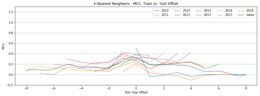
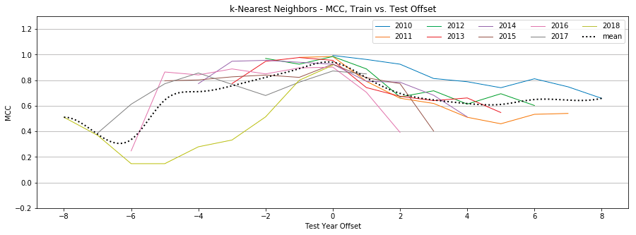
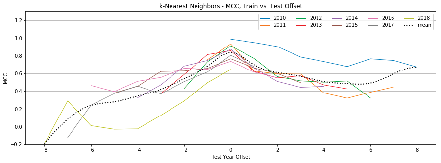
Figure 9: k-Nearest-Neighbors, MCC by year, Tweet-Only vs. User-Only vs. All Features
Logistic Regression
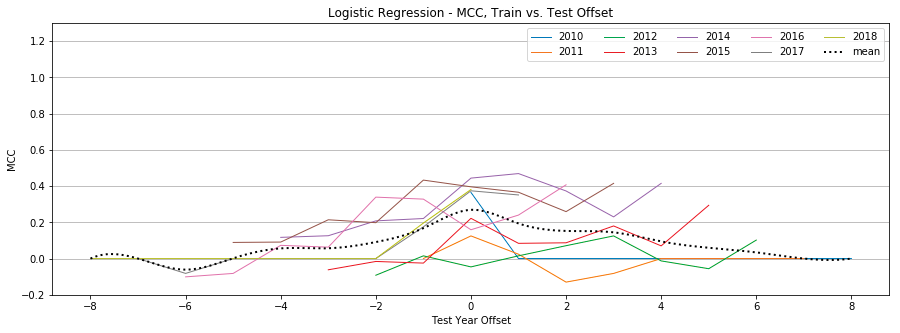
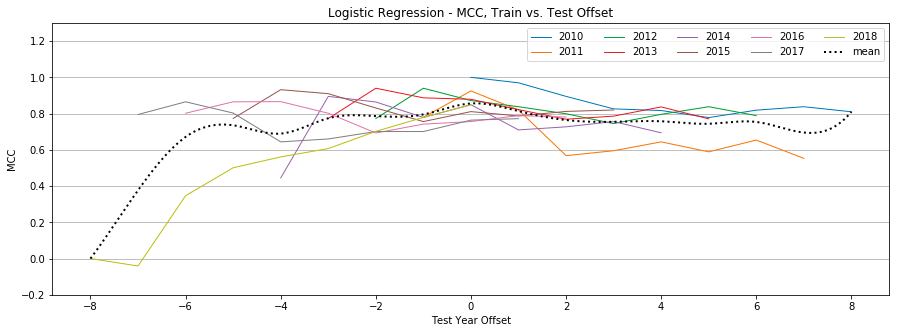
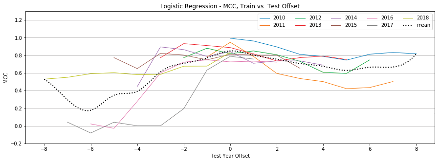
Figure 10: Logistic Regression, MCC by year, Tweet-Only vs. User-Only vs. All Features
SVC


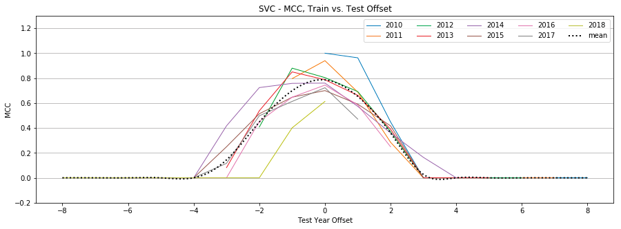
Figure 11: SVC, MCC by year, Tweet-Only vs. User-Only vs. All Features
MLP
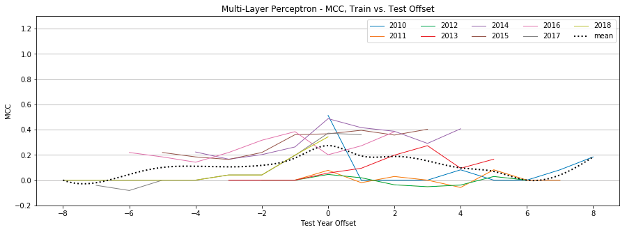
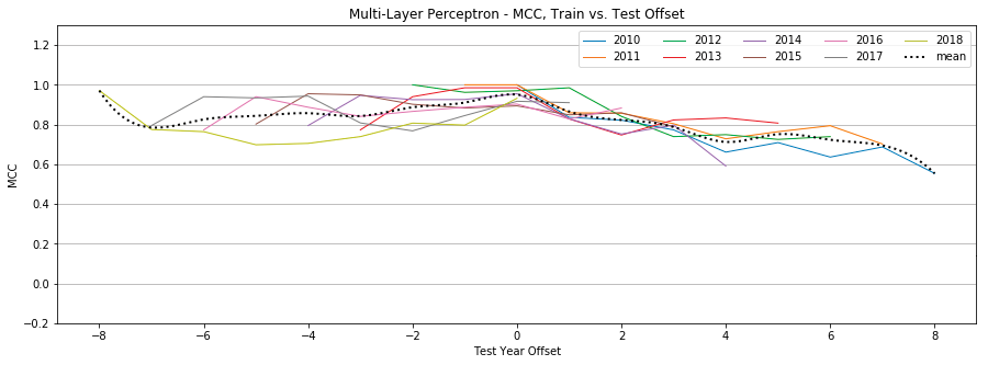
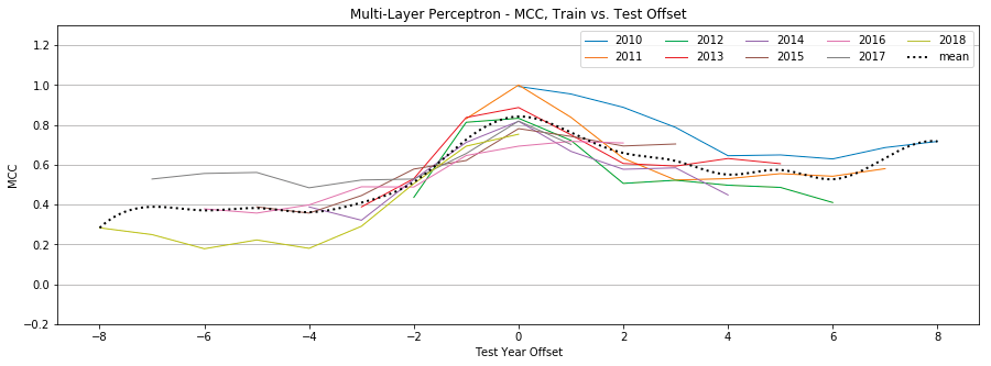
Figure 12: Multi-Layer Perceptron, MCC by year, Tweet-Only vs. User-Only vs. All Features
Decision Trees
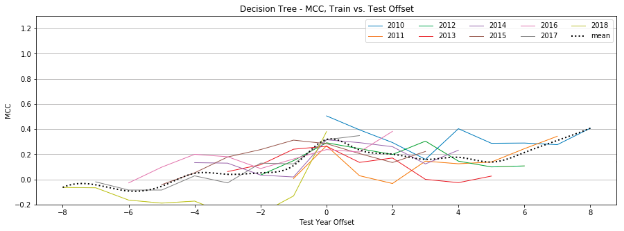
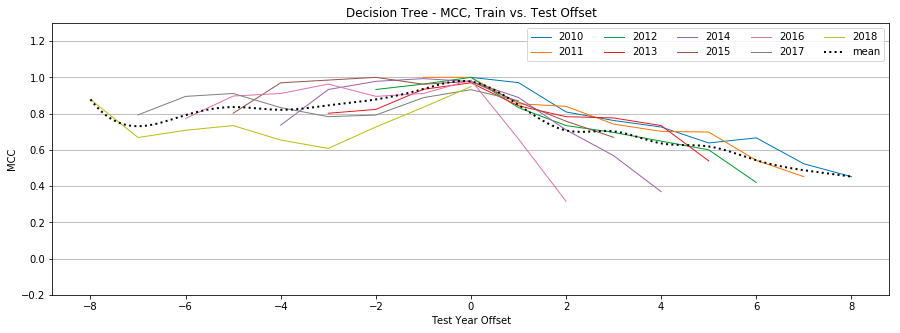
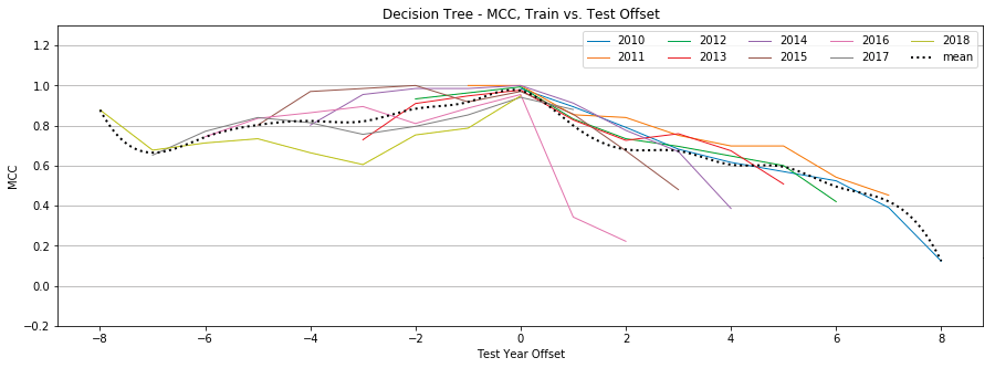
Figure 13: Decision Tree, MCC by year, Tweet-Only vs. User-Only vs. All Features
Random Forest
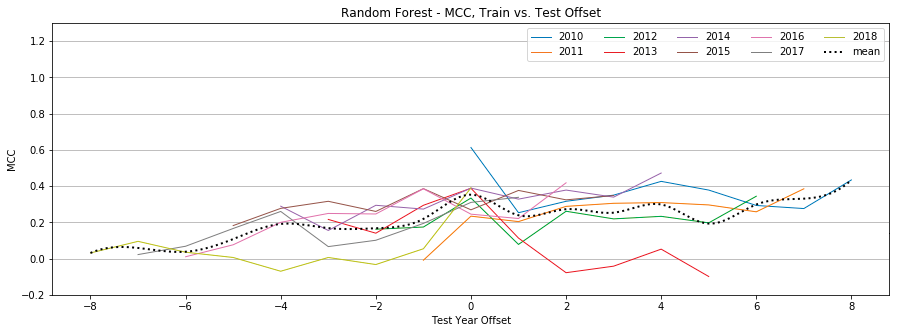
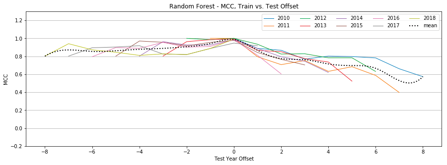
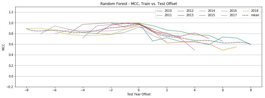
Figure 14: Random Forest, MCC by year, Tweet-Only vs. User-Only vs. All Features
Gradient Boosting
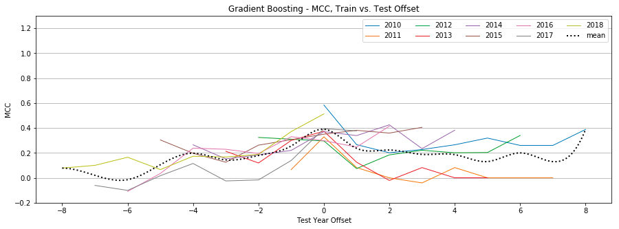
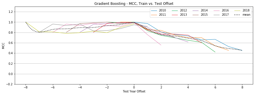
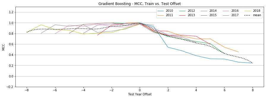
Figure 15: Gradient Boosting, MCC by year, Tweet-Only vs. User-Only vs. All Features
References
- Bailey, M., Cooke, E., Jahanian, F., Xu, Y., & Karir, M. (2009). A Survey of Botnet Technology and Defenses. In 2009 Cybersecurity Applications Technology Conference for Homeland Security (pp. 299–304). https://doi.org/10.1109/CATCH.2009.40
- Boughorbel, S., Jarray, F., & El-Anbari, M. (2017). Optimal classifier for imbalanced data using Matthews Correlation Coefficient metric. PLOS ONE, 12(6), e0177678. https://doi.org/10.1371/journal.pone.0177678
- Chu, Z., Gianvecchio, S., Wang, H., & Jajodia, S. (2010). Who is Tweeting on Twitter: Human, Bot, or Cyborg? In Proceedings of the 26th Annual Computer Security Applications Conference (pp. 21–30). New York, NY, USA: ACM. https://doi.org/10.1145/1920261.1920265
- Cooke, E., Jahanian, F., & McPherson, D. (2005). The Zombie Roundup: Understanding, Detecting, and Disrupting Botnets. In Proceedings of the Steps to Reducing Unwanted Traffic on the Internet on Steps to Reducing Unwanted Traffic on the Internet Workshop (pp. 6–6). Berkeley, CA, USA: USENIX Association. Retrieved from http://dl.acm.org/citation.cfm?id=1251282.1251288
- Echeverría, J., & Zhou, S. (2017). Discovery, Retrieval, and Analysis of “Star Wars” botnet in Twitter. ArXiv:1701.02405 [Cs]. Retrieved from http://arxiv.org/abs/1701.02405
- Gu, G., Zhang, J., & Lee, W. (2008). BotSniffer: Detecting Botnet Command and Control Channels in Network Traffic.
- Hua, W., & Zhang, Y. (2013). Threshold and Associative Based Classification for Social Spam Profile Detection on Twitter. In 2013 Ninth International Conference on Semantics, Knowledge and Grids (pp. 113–120). https://doi.org/10.1109/SKG.2013.15
- Jose Nazario. (2009, August 13). Twitter-based Botnet Command Channel. Retrieved May 27, 2018, from https://asert.arbornetworks.com/twitter-based-botnet-command-channel/
- Kartaltepe, E. J., Morales, J. A., Xu, S., & Sandhu, R. (2010). Social Network-Based Botnet Command-and-Control: Emerging Threats and Countermeasures. In J. Zhou & M. Yung (Eds.), Applied Cryptography and Network Security (pp. 511–528). Berlin, Heidelberg: Springer Berlin Heidelberg.
- Nagaraja, S., Houmansadr, A., Piyawongwisal, P., Singh, V., Agarwal, P., & Borisov, N. (2011). Stegobot: A Covert Social Network Botnet. In T. Filler, T. Pevný, S. Craver, & A. Ker (Eds.), Information Hiding (pp. 299–313). Berlin, Heidelberg: Springer Berlin Heidelberg.
- Natarajan, V., Sheen, S., & Anitha, R. (2012). Detection of StegoBot: A Covert Social Network Botnet. In Proceedings of the First International Conference on Security of Internet of Things (pp. 36–41). New York, NY, USA: ACM. https://doi.org/10.1145/2490428.2490433
- Pantic, N., & Husain, M. I. (2015). Covert Botnet Command and Control Using Twitter. In Proceedings of the 31st Annual Computer Security Applications Conference (pp. 171–180). New York, NY, USA: ACM. https://doi.org/10.1145/2818000.2818047
- Rodríguez-Gómez, R. A., Maciá-Fernández, G., & García-Teodoro, P. (2013). Survey and Taxonomy of Botnet Research Through Life-cycle. ACM Comput. Surv., 45(4), 45:1–45:33. https://doi.org/10.1145/2501654.2501659
- Stamp, M., Singh, A., H. Toderici, A., & Ross, K. (2013). Social Networking for Botnet Command and Control. International Journal of Computer Network and Information Security, 5, 11–17.
- Vania, J., Meniya, A., & Jethva, H. (2013). A Review on Botnet and Detection Technique. International Journal of Computer Trends and Technology, 4(1), 23–29.